Climate 2: Rivers and Erosion

I’m doing this a little out of order. Why groundwater and erosion first? Modeling the water layer on and in the ground is an isolated section of climate simulation. Whereas the air modeling has interdependent parts (radiation, convection, etc.), the groundwater system is self-contained except for precipitation and evaporation. I can easily implement a dummy precipitation/evaporation system.

Second, the groundwater system is a good warm up for the air modeling. There are a lot of similarities between how water and air layers are modeled: they are both grid systems moving fluids around based on pressure. The water system is much simpler because water is incompressible and water pressure is solely dependent on depth. Water also moves more slowly and there’s less of it.

Feel free to skip to the Results section.

Table of Contents

Introduction and Science

T.C. Winter, J.W. Harvey, O.L. Franke, and W.M. Alley – Ground Water And Surface Water A Single Resource. U.S. Geological Survey Circular 1139.

Most groundwater is underground in aquifer layers, or zones of saturation. The top of the aquifer is referred to as the water table. Despite how they are often depicted, aquifers are generally not underground rivers. They’re really layers of porous rock, like a layer of sponge between layers of non-porous rock. As you might imagine, it takes a long time for water to move through these porous rock layers, sometimes with speeds on the order of centimeters per year.

In some areas, the water table is above the surface of the ground. Then you get surfacewater, like rivers and lakes. Rarely, when the surface is non-porous, surfacewater can occur even when the water table is far below ground. Water aboveground moves much faster, up to the order of meters per second. Note: Surfacewater is not a word but that’s what I’ll call all water aboveground.

Goals

I have three goals for the groundwater and erosion system.

Rivers and Lakes

I want to generate rivers and lakes from the groundwater simulation. This gets a little tricky due to the extremely low resolution of my map. For example, if my tiles are 50 km wide, then I can’t realistically model rivers, since rivers are much narrower than 50 km. So I’ll have to use some heuristics and hand-waving to draw rivers from my groundwater simulation. Still, a chain of adjacent tiles with lots of surface water flowing over them should create a river, and tiles with a large amount of standing water should be lakes.

Terrain Shaping

I’d like the erosion system to create river basins. As mentioned above, this may be tricky due to the low resolution of the map.

Biome Identification

When I do biome identification, I’d like to use the groundwater system to identify areas saturated with water as wetlands. This isn’t very important because I can always just fall back on using the precipitation levels to identify wetlands.

All right, let’s look at some literature on computational erosion models.

Research/Literature

Most of my model is based on:

Xing Mei, Philippe Decaudin, Bao-Gang Hu. Fast Hydraulic Erosion Simulation and Visualization on GPU. Marc Alexa and Steven J. Gortler and Tao Ju. PG ’07 – 15th Pacific Conference on Computer Graphics and Applications, Oct 2007, Maui, United States. IEEE, pp.47-56, 2007, Pacific Graphics 2007. <10.1109/PG.2007.15>. https://hal.inria.fr/inria-00402079.

I’ll try to write everything out so you don’t need to read the paper, as I do have some differences, but I still recommend reading the paper (and some of its references). It’s a pretty easy read.

A much older paper that’s also relatively readable:

F. Musgrave, C. Kolb, and R. Mace. The Synthesis and Rendering of Eroded Fractal Terrains. Computer Graphics, Vol. 23, Num. 3, Jul 1989.

The Model Design

Surfacewater lateral flow: Four outflows are calculated for each tile.

At each tick, the following is calculated:

Precipitation adds to surface water
Evaporation subtracts from surface water
Surfacewater drains into groundwater if there is room
Excess groundwater is moved to surfacewater
Lateral surfacewater movement. At each tile:
1. The outflow velocity in all four directions is calculated based on pressure differential
2. Outflow velocities are capped at a speed limit
3. Water height is recalculated from the sum of all outflows and inflows
Lateral groundwater movement is similar to surfacewater movement
Sediment is picked up or deposited at each tile based on the current dissolved sediment compared to the sediment capacity
Lateral sediment movement is calculated using a semi-Lagrangian approach

I store surfacewater and groundwater as heights since it’s trivial to calculate the volume by multiplying by the constant tile area.

Precipitation and Evaporation

For now, I’ll use a trivial precipitation and evaporation system. Eventually (not in this post) this will be replaced with a full water cycle simulation.

The water layer itself will have two sublayers: groundwater and surfacewater. Rain (for now I’m not considering frozen precipitation) is all added to surfacewater.

Surface-Groundwater Exchange

The groundwater sublayer has a maximum amount of water it can store. If the groundwater in a tile ever exceeds its maximum capacity, the excess groundwater is immediately moved to the surface. This models when the water table is higher than the ground.

If the groundwater in a tile is below the tile’s groundwater capacity, then any surfacewater slowly drains into the groundwater layer. The exact function governing the speed of draining can be experimented with.

Note: Currently I have a constant groundwater sublayer capacity. I don’t do very much with it. In the future, if I do more underground modeling, I’d like to have it conform to the following image, where the bottom depth of the aquifer is independent of local changes in elevation.

Lateral Water Movement

This is the complicated bit for which I recommend also reading the “Fast Hydraulic Erosion” paper. I’ll explain the simulation for surface water first.

All the tiles are treated as closed tanks connected by pipes. The pipes connect the bottom of the tanks.

Side view of two adjacent tiles connected by a pipe

The velocity in the pipes is governed by the pressure differential between the tiles. Water pressure is governed by the height of water above it:

$P = \rho gh$

I care about the difference in water pressure. In this scenario, the difference in water pressure depends solely on the difference in the height of the water in the two adjacent tiles. Note that this height difference includes any difference in the ground elevation.

$\Delta P_{1,2} = \rho_1 g_1 h_1 - \rho_2 g_2 h_2$

$\Delta P_{1,2} = \rho g (h_1 - h_2)$

where each h is the sum of the terrain elevation and the surface water height.

At time t = 0, the velocity in every pipe starts at 0. After t = 0, the pipe velocity is accelerated by the pressure differential. The velocity update equation for a pipe is:

$f_{t+\Delta t} = f_t + \Delta t * \frac{g * \Delta h}{l}$

where l is the pipe length, which is the side length of a tile

I only want the outflow, so I’ll remove negative velocities. Inflows will be calculated from adjacent tiles’ outflows.

$f_{t+\Delta t} = max \left( 0, f_t + \Delta t * \frac{g * \Delta h}{l} \right)$

There’s a problem: what if my total outflow exceeds the amount of water on the tile? In this case I need to scale down all the outflow from the tile (this is why I focus on calculating outflows at every tile). From the pipe velocity, I can calculate the amount of water transferred between tiles during a tick.

$\Delta V = Q * \Delta t = f * A * \Delta t$

where Q is the volumetric flowrate and A is the pipe cross-sectional area

Note: The pipe cross-sectional area A is an arbitrary parameter (since these are imaginary pipes). It is useful to control how fast water moves around in the simulation. Reducing the pipe area size is useful for offsetting some of the undesirable effects of having such large tiles.

So if $A * \Delta t * \sum f(x,y)^i > waterCurrentlyOnTile$ , I need to scale down all four outflows by a factor of at least $K = \frac{waterCurrentlyOnTile}{totalUnscaledOutflow}$ .

At each tick, the water height at each tile is changed by adding the total inflows from adjacent tiles and subtracting the outflows from the current tile.

The change in water height at a tile is equal to the four inflows minus the four outflows.

Groundwater lateral movement is much the same, except it has a much smaller pipe area to simulate the filtering effect and slow movement of groundwater.

Finally, whenever water flows into the ocean, it’s destroyed. I don’t run any groundwater simulation on ocean tiles.

Sediment Dissolution and Deposition

Whenever surfacewater is present on a tile, the surfacewater can either pick up or deposit sediment. The sediment capacity of the surfacewater on Tile(x,y) is given by the following equation:

$C(x,y) = K_c * sin(a(x,y)) * |v(x,y)|$

where $K_c$ is the sediment capacity (solubility limit) constant, $a$ is the local tilt angle (between 0 and $\pi / 2$ ), and $|v(x,y)|$ is the horizontal water speed.

As you can see, the sediment capacity increases when the terrain is steeper and when the water velocity is higher. This has an issue where very flat terrain has nearly zero erosion. I can fix this by adding a minimum sediment capacity.

$C(x,y) = K_c * max(minSedi, sin(a(x,y)) * |v(x,y)|)$

Note: At this point, I diverge a bit from the Fast Erosion paper. Their deposition/dissolution equations don’t take into account the timestep $\Delta t$ , which I am unable to explain.

At each tile, if the suspended sediment $s$ exceeds the sediment capacity $C$ , then sediment is deposited. If $s < C$ , then sediment is dissolved. Therefore, the change in suspended sediment is given by:

$ds = K(C-s)dt$

where K is like a dissolution rate constant (Note: the paper uses separate constants for dissolution and deposition, whereas I use the same constant)

Integrating:

$\int_{s_0}^{s_t} \frac{ds}{s-C} = \int_{t_0}^{t} -K dt$

$\ln(\frac{s_t - C}{s_0 - C}) = -K(t-t_0)$

$s_t = C + (s_0 - C) e^{-K(t-t_0)}$

$\Delta s = (C - s_0) \left( 1-e^{-K\Delta t} \right)$

Note: Although the exponential function is expensive, it is independent of the location, so it only has to be calculated once per tick.

This change in sediment $\Delta s$ is added to the suspended sediment and subtracted from the tile elevation. There is some leeway here in how exactly the sediment concentration is tracked and converted to elevation. For the most Science, the actual amount of sediment should be tracked and converted to elevation in order to keep this step mass conservative. I used a less rigorous approach that let me exaggerate the elevation changes to speed up the erosion process.

Sediment Movement: Semi-Lagrangian

Despite the fancy name, this method is actually very simple. This is again the approach taken by Mei et al.

To model the movement of sediment dissolved/suspended in water, at every tile I take an Eulerian step back in time. Basically, I travel backwards along the tile’s water velocity vector and take the sediment value from there.

Example:

At Tile(x = 5, y = 3), if the timestep is 1 second and the water velocity at the tile is (1, 2) m/s.

Eulerian step back in time: $(5, 3) - 1 * (1, 2) = (4, 1)$ . So the sediment value at Tile(5,3) at $t=t_0 + 1$ is whatever the sediment value was at Tile(4, 1) at $t=t_0$ . Since the Eulerian step back in time usually does not result in perfect integer coordinates, the sediment value is interpolated from the surrounding tiles.

Note: As always, this step needs a “speed cap” to prevent instabilities (ideally the Eulerian step back in time would always be less than a full tile. Definitely don’t want it to move 50 tiles at at time). As long as the speed cap from the water flow rate section is low enough, I don’t need to add another one here.

Results and Troubleshooting

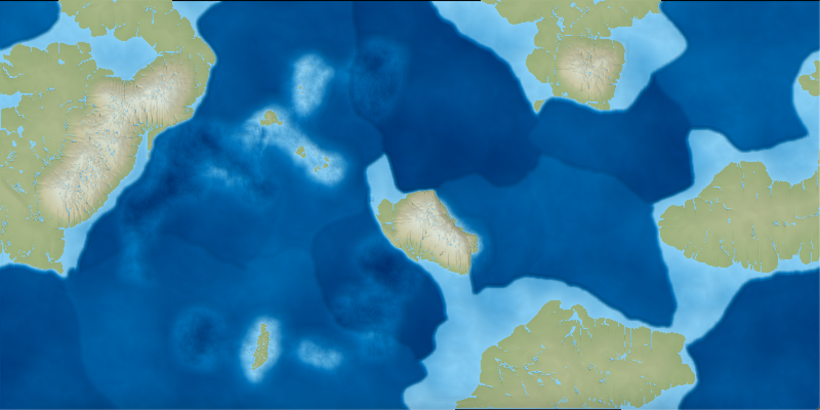
I apologize for using the same rendering color for both surfacewater (rivers, lakes) and shallow ocean (continental shelves). Also, as a note, I’m rendering surfacewater where the volumetric flowrate over a tile is greater than an arbitrary threshold. This is not necessarily the best way to identify rivers/lakes.

This is the first stable version of the erosion simulation. The mountainsides are looking pretty eroded. It’s not perfect, but, given the tile size involved, I think that’s the best I can hope for. There are a couple of issues though.

First, the plains and the central mountain areas aren’t getting very eroded. There are a few levers I can pull to alleviate this. The easiest one is to increase the minimum sediment capacity so that slow-moving water over flat areas will carry more sediment.

Bumping up sediment-carrying capacity by factor of 10 causes entire continents to erode

Yikes. After some experimentation, it seems that whole continents will erode before the hint of a river will manifest in the flatter areas. This requires a bit more careful analysis.

There are a few things going on here. First, water is rushing very fast down the sides of the mountains, then it gathers at the foot of the mountain ranges, but it doesn’t make it out to sea.

The water rushing down the mountainsides probably indicates that my maximum water velocity is too high.

After going back and comparing units, it turns out that my maximum water velocity is over 200 m/s, which is indeed too high. I’ll reduce it to a more realistic 5 m/s. Also, I’m naively capping the x-velocity and y-velocity independently. This both allows greater diagonal velocity (up to $5\sqrt{2}$ ) and means many too-fast velocities are shifted to a perfectly diagonal direction. Instead, I’ll change the speed cap function to calculate the magnitude of the velocity vector (which unfortunately requires an expensive square root function). These changes reduce the erosion of the mountainsides and increase erosion in the main mountain areas, but they don’t increase erosion in the plains areas.

The water gathers at the foot of the mountain ranges but doesn’t make it out to sea. That means one of two things: either the water is spreading out into a thin, even layer over the plains, or the water is evaporating before it makes it very far. I suspect it’s the latter, since I’m using an arbitrary guess for the evaporation rate. Although, it’s also possible this is an unforeseen symptom of too-large tile sizes. I hope that’s not the case.

According to the many pool owners online, water evaporates at roughly 1/2 cm per day. That translates to 5e-8 m/s. I was using 1e-5 m/s. That’s pretty far off. I’ll update the evaporation rate and tweak the precipitation numbers to keep the simulation stable. Let’s see if the reduced evaporation makes a difference.

Groundwater/erosion after improving evaporation and max water speed

Hey, those kind of look like rivers. They are too wide, which likely is partially caused by my massive tile size, and I’ve lost the mountainous rivers, but that’s probably related to my surfacewater-rendering threshold.

After more tweaking of the various constants and occasional debugging and cleaning, it looks like this.

Erosion system after some number of simulated years.

In the above image, rivers/lakes were “detected” by coloring land light blue whenever the surfacewater height was greater than 1 meter.

TODO

There is still an issue I would like to investigate: there is a grid artifact (erosion prefers to occur along horizontal or vertical lines, becoming more obvious with a larger sediment dissolution rate constant). This could have a lot of causes. For now, it seems to be minimized by using a low erosion dissolution rate constant and running more ticks.

Also, when I reach the full water cycle and integrate this erosion system, I’ll revisit the river formation to make them look more river-y. I may also need to revisit my mountain generation algorithm to work better with the erosion system.

Next Up

I’ll start on the climate model with insolation and radiation.